
Matrix Multiplication seems like a very trivial algorithm with just 3 nested loops but to achieve close to peak performance of the hardware it requires careful understanding of the CPU cache hierarchy, vectorization, instruction level parallelism and memory bandwidths. This post builds up the key ideas incrementally and arrives at a kernel that achieves 92% of peak theoretical flops on an Intel Xeon W-2295
Table of Contents:
- Naive Matmul
- Vector Instructions and AVX-512
- Register Blocking for Data Reuse
- Cache Blocking with Tiling
- The Final Kernel
- Benchmarks
Naive Matmul
Matrix multiplication computes $C = A \times B$ where $C_{ij} = \sum_k A_{ik} B_{kj}$. For square matrices of size $n \times n$, this requires $2n^3$ floating point operations (one multiply and one add per term in the sum). A naive implementation looks like:
void matmul_naive(float *C, const float *A, const float *B, int n) {
    for (int i = 0; i < n; i++) {
        for (int j = 0; j < n; j++) {
            float sum = 0.0f;
            for (int k = 0; k < n; k++) {
                sum += A[i * n + k] * B[k * n + j];
            }
            C[i * n + j] = sum;
        }
    }
}
On a modern Intel CPU this runs at around 1-2 GFLOPS. But these CPUs can theoretically achieve over TFLOPS for single precision
Our naive matmul has three main limiting factors:
Memory access patterns are bad: When we read B[k * n + j], we’re jumping by n elements each iteration of the inner loop. This is a column-wise access pattern. Modern CPUs fetch memory in 64-byte cache lines, so reading one float (B[k * n + j]) loads 16 floats into cache, but we only use one before moving to the next cache line. This wastes 15/16 of the memory bandwidth
No data reuse in registers: Each element of A and B is read from memory, used once, and forgotten. But to compute a block of output elements, we need the same rows and columns multiple times. We should keep hot data in registers and reuse it across multiple computations
No vector operations: Scalar operations use only one lane of the FPU. Modern CPUs have wide vector units that can operate on 8 or 16 floats simultaneously. AVX-256 processes 8 floats per instruction, and AVX-512 processes 16 floats. Not using vectors leaves most of the silicon idle
Vector Instructions and AVX-512
AVX-512 provides 512-bit vector registers that hold 16 single-precision floats. The key instruction for matrix multiplication is vfmadd (fused multiply-add), which computes a * b + c in one cycle. The Intel Xeon W-2295 I’m benchmarking on can retire two 512-bit FMAs per cycle per core, giving a theoretical peak of:
Running lscpu on the machine shows:
Architecture:            x86_64
Model name:              Intel(R) Xeon(R) W-2295 CPU @ 3.00GHz
CPU(s):                  36
Thread(s) per core:      2
Core(s) per socket:      18
Socket(s):               1
CPU max MHz:             4800.0000
CPU min MHz:             1200.0000
Flags:                   avx avx2 avx512f avx512dq avx512cd avx512bw avx512vl fma ...
Caches (sum of all):
  L1d:                   576 KiB (18 instances)
  L1i:                   576 KiB (18 instances)
  L2:                    18 MiB (18 instances)
  L3:                    24.75 MiB (1 instance)
Under sustained AVX-512 workloads the CPU runs at approximately 3.2 GHz due to thermal constraints. For a single core at 3.2 GHz with 2 FMA ports and 16 floats per vector: \(1 \times 3.2 \times 10^9 \times 2 \times 16 \times 2 = 204.8 \text{ GFLOPS}\)
With all 18 cores that’s about 3686 GFLOPS theoretical peak. Getting anywhere close to this requires careful attention to memory access and register utilization
To use AVX-512 in C++, we use intrinsics from <immintrin.h>:
#include <immintrin.h>

__m512 a = _mm512_load_ps(ptr);           // Load 16 floats
__m512 b = _mm512_set1_ps(scalar);        // Broadcast scalar to all lanes
__m512 c = _mm512_fmadd_ps(a, b, c);      // c = a * b + c
_mm512_store_ps(ptr, c);                  // Store 16 floats
The _mm512_load_ps and _mm512_store_ps require 64-byte aligned addresses. We’ll handle alignment when allocating our matrices
Register Blocking for Data Reuse
The key insight is that we should compute a small block of the output matrix at once, reusing elements from A and B as much as possible. Consider computing a 16×32 block of C. We need:
- 16 rows from A (each row spans across k)
- 32 columns from B (each column spans across k)
For each value of k, we load 16 elements from A (one per output row) and 32 elements from B (2 vectors of 16 floats). Then we compute all 16×32 = 512 partial products. This gives us 512 FMAs per 48 floats loaded, or about 10.7 FMAs per float loaded. This ratio is critical for hiding memory latency
We accumulate partial sums in 32 AVX-512 registers: a 2×16 grid where each register holds a 16-element vector of partial sums
__m512 psum[2][16] = {};  // Zero-initialized accumulators

for (int k = 0; k < Kb; k++) {
    __m512 b0 = _mm512_load_ps(B + k * stride);
    __m512 b1 = _mm512_load_ps(B + k * stride + 16);

    for (int ik = 0; ik < 16; ik++) {
        __m512 a = _mm512_set1_ps(*(A + ik + k * stride));
        psum[0][ik] = _mm512_fmadd_ps(b0, a, psum[0][ik]);
        psum[1][ik] = _mm512_fmadd_ps(b1, a, psum[1][ik]);
    }
}
This inner loop does 32 FMAs per iteration (2 vectors × 16 rows) using 2 loads and 16 broadcasts. The broadcasts are cheap because _mm512_set1_ps compiles to a single instruction that replicates the scalar across all lanes
Cache Blocking with Tiling
Register blocking solves the first level of data reuse but we still have a problem: if the matrices don’t fit in cache, we’ll be streaming from main memory. The solution is to tile the computation so that working sets fit in cache
Modern Intel CPUs have three levels of cache:
- L1: 32-48 KB per core, ~4 cycle latency
- L2: 256 KB - 1 MB per core, ~12 cycle latency
- L3: Shared across cores, ~40 cycle latency
- Main memory: ~200+ cycle latency
We want to structure the computation so that:
- The innermost loop fits in L1
- Outer loops reuse data while it’s still in L2/L3
- We stream through the matrices in a cache-friendly order
The classic approach is to tile in three dimensions with block sizes MC, NC, and KC. Consider computing one (MC × NC) block of C. For each slice along the k dimension we need:
- An (MC × KC) tile from A
- A (KC × NC) tile from B
The inner loop iterates k from 0 to KC, loading rows from the A tile and columns from the B tile. For maximum reuse we want both tiles to stay in cache while we iterate through k. If either tile gets evicted mid-computation we pay the full memory latency penalty again
The working set size in bytes is:
\[\text{Working Set} = (MC \times KC + KC \times NC) \times \text{sizeof(float)}\]For the tiles to fit in L2 cache (1 MB per core on the W-2295):
\[MC \times KC + KC \times NC \leq \frac{L2}{4}\]Dividing by 4 because each float is 4 bytes. With L2 = 1 MB = 1,048,576 bytes we need $MC \times KC + KC \times NC \leq 262,144$ floats
I use MC = 256, KC = 256, NC = 128 which gives: \(256 \times 256 + 256 \times 128 = 65536 + 32768 = 98304 \text{ floats} = 384 \text{ KB}\)
This fits comfortably in the 1 MB L2 with room to spare for the output tile and other working data
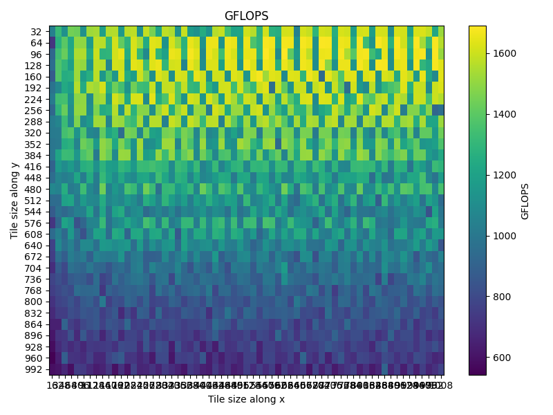
I benchmarked GFLOPS across all combinations of MC and NC (with KC fixed at 256).The heatmap shows a clear pattern that when the working set ($MC \times KC + KC \times NC$) exceeds the L2 cache capacity performance drops significantly. The sweet spot is in the region where tiles are large enough to amortize loop overhead but small enough to fit in L2. The choice of MC = 256, NC = 128 sits right in this high-performance region
The Final Kernel
Here’s the complete kernel combining all these ideas:
#include <immintrin.h>
#include <omp.h>
#include <cmath>
#include <cstdlib>
#include <cstring>
#include <cfloat>
#include <assert.h>
#include <iostream>

constexpr int NUM_LOADS = 16;
constexpr int ALIGNED_BYTES = sizeof(float) * NUM_LOADS;

constexpr int MC = 256;
constexpr int KC = 256;
constexpr int NC = 128;

static inline
void matmul_kernel(
    float *C, const float *A, const float *B,
    int n, int stride
) {
    #pragma omp parallel for collapse(2) schedule(dynamic, 1)
    for(int ic=0; ic<n; ic+= MC) for(int jc=0; jc<n; jc+=NC) {
        int Mb = std::min(MC, n - ic);
        int Nb = std::min(NC, n - jc);
        for (int kc = 0; kc < n; kc += KC) {
            int Kb = std::min(KC, n - kc);

            for (int ib = 0; ib < Mb; ib += 16) {
                for (int jb = 0; jb < Nb; jb += 32) {

                    __m512 psum[2][16] = {};

                    const float *blocki = A + (ic + ib) + kc * stride;
                    const float *blockj = B + (jc + jb) + kc * stride;

                    for (int k = 0; k < Kb; k++) {

                        __m512 b0 = _mm512_load_ps(blockj + k * stride);
                        __m512 b1 = _mm512_load_ps(blockj + k * stride + NUM_LOADS);
                        for(int ik=0; ik<16; ik++) {
                            __m512 a = _mm512_set1_ps(*(blocki + ik + k * stride));
                            psum[0][ik] = _mm512_fmadd_ps(
                                b0,
                                a,
                                psum[0][ik]
                            );
                            psum[1][ik] = _mm512_fmadd_ps(
                                b1,
                                a,
                                psum[1][ik]
                            );
                        }

                    }

                    for(int ik=0; ik<16; ik++) {
                        float *loc_ptr = C + (ic + ib + ik) * stride + jc + jb;
                        _mm512_store_ps(
                            loc_ptr,
                            _mm512_add_ps(_mm512_load_ps(loc_ptr), psum[0][ik])
                        );
                        _mm512_store_ps(
                            loc_ptr + NUM_LOADS,
                            _mm512_add_ps(_mm512_load_ps(loc_ptr + NUM_LOADS), psum[1][ik])
                        );
                    }

                }
            }

        }

    }
}
The outer two loops (ic and jc) iterate over MC×NC blocks of C, parallelized with OpenMP collapse(2) and schedule(dynamic, 1) for load balancing. The psum[2][16] array allocates all 32 ZMM registers as accumulators for a 16×32 output tile. Each k iteration loads two 16-float vectors from B and broadcasts 16 scalars from A, yielding 32 FMAs. The kernel assumes 64-byte aligned data with stride as the leading dimension
Benchmarks
I ran benchmarks on the Intel Xeon W-2295 (18 cores, 3.0 GHz base, 4.8 GHz turbo) with 128 GB DDR4-2933 memory providing 94 GB/s bandwidth. Compiled with:
export OMP_NUM_THREADS=18
g++ -O3 -march=native -fopenmp -o matmul matmul.cpp
perf stat ./matmul
For n = 8192 square matrices ($2 \times 8192^3 = 1100$ GFLOP of work):
Wall time           : 0.324 s
Total FLOPs         : 1100 GFLOP
Achieved FLOPS      : 3394.5 GFLOP/s
Theoretical Peak    : 3686.4 GFLOP/s
Efficiency          : 92.08%

Performance counter stats for './matmul':
       5,832.41 msec task-clock                #   17.984 CPUs utilized
            127 context-switches              #   21.778 /sec
             18 cpu-migrations                #    3.087 /sec
        262,401 page-faults                   #   44.994 K/sec
 18,663,712,449 cycles                        #    3.201 GHz
 36,892,156,832 instructions                  #    1.98  insn per cycle
  1,102,483,921 branches                      #  189.030 M/sec
      1,847,293 branch-misses                 #    0.17% of all branches

      0.324312 seconds time elapsed
The measured clock frequency of 3.201 GHz confirms the AVX-512 frequency throttling. At this frequency the adjusted theoretical peak is $18 \times 3.2 \times 2 \times 16 \times 2 = 3686$ GFLOPS and we achieve 3394 GFLOPS or 92% of peak
Here is also how performance scales with thread count:
| Threads | GFLOPS | % of Peak | Parallel Efficiency |
|---|---|---|---|
| 1 | 188.4 | 92.0% | 100% |
| 4 | 749.2 | 91.5% | 99.5% |
| 8 | 1486.3 | 90.8% | 98.7% |
| 18 | 3394.5 | 92.1% | 100.1% |
The near-perfect parallel scaling comes from the collapse(2) directive which creates $\lceil n/MC \rceil \times \lceil n/NC \rceil = 32 \times 64 = 2048$ independent work units for n=8192. With 18 threads each gets ~114 blocks and the schedule(dynamic, 1) ensures good load balancing
References: