LLMs are created for different tasks and thus they have having varying capabilities and efficiencies for a particular input query, while certain llms are trained to answer simple questions while being cost efficient certain are trained to solve complex IMO problems and cost is not in consideration for such tasks. However while serving llms queries ranging from simple to complex tasks need to be answered and using a single model to answer them is not only infeasible but also damages the performance of the output generated.

To avoid this LLMs are ensembled and queries are routed via a router to the most suitable llm. This routing depends on an accurate understanding of each of the llms performance and query on certain tasks and queries.

In Performance-Efficiency optimized routing the router builds this understanding from a set $\mathcal{D}$ of query–answer pairs. Each query $d \in \mathcal{D}$ is encoded into a semantic vector using a text embedding model. Then these embeddings are clustered into $k$ clusters using any clustering algorithm giving us clusters $\mathcal{C}={c_{1}, c_{2}, …, c_{k}}$, where each cluster has semantically coherant queries.

Then for each of $\mathcal{M}$ models we evaluate the performance and efficiency on each cluster giving us performance profiles $p^{i}={p_{1}^{i}, p_{2}^{i}, …, p_{k}^{i}}$ and efficiency profiles $q^{i}={q_{1}^{i}, q_{2}^{i}, …, q_{k}^{i}}$ for model $i \in \mathcal{M}$. They measure performance by computing accuracy across the cluster and efficiency is measured in terms of total cost incurred by model $i$ to answer all queries in cluster $c_{j}$.

Then they compute the performance–efficiency score for model $i$ on cluster $j$ as

\[x_{j}^{i} = \alpha \bar{p}_{j}^{i} + (1 - \alpha) (1 - \bar{q}_{j}^{i})\]

here $\bar{p}_j^i$, $\bar{q}_j^i$ are normalized performance and efficiency profiles respectively computed from the max and min scores across the profiles and $\alpha$ controls the trade off between performance and efficiency.

At test time for an input query the $top$-${p}$ closest clusters in the embedding space are computed from encoding the query using a text embedding model. The query is then routed to the model with the highest aggregated cluster wise performance–efficiency score.

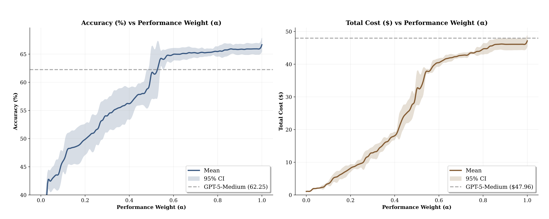Figure 1: Effects of the trade-off parameter $\alpha$ on the performance and efficiency. A greater value of $\alpha$ prioritizes performance over efficiency. The increase in performance is usually accompanied with increase in cost (source: Zhang et al. 2025).

They note their routing outperforms all individual models for higher values of $\alpha$ when performance is prioritized. Thus at levels comparable to the performance of the strongest model the routing achieves significantly lower cost.

Arch Router reframes routing as preference alignment: given a natural-language policy set, pick the policy that best matches the user’s current intent, then map that policy to a model. Concretely, define a set of route policies $\mathcal{C}={c_1,\dots,c_k}$, each $c^i=(n^i,d^i)$ with an identifier $n^i$ and a natural-language description $d^i$. Policies are written in a Domain–Action taxonomy: Domain (for example legal, finance) captures topic; Action (for example summarization, code generation) captures operation. A separate mapping $T:\mathcal{C}\to\mathcal{M}$ assigns each policy to a concrete model. The router $F:(q,\mathcal{C})\to c$ selects a policy from text alone; model choice is then

\[R(q)= (T\circ F)(q,\mathcal{C}).\]

This decoupling means adding or swapping models is an edit to $T$, not a retrain of $F$. Ambiguous requests degrade gracefully: if Action is fuzzy, the system can still resolve Domain.

Arch Router is a compact 1.5B generative LM trained to emit the policy identifier for a structured prompt $x$ that contains the full policy set $\mathcal{C}$ and the conversation (multi-turn history, not just the last message). Training minimizes cross-entropy over $(x,c_{\text{true}})$:

\[\min_{\mathcal{F}_{\text{Arch}}}\ \mathcal{L}\big(\mathcal{F}_{\text{Arch}}(x),\,c_{\text{true}}\big).\]

Because $\mathcal{C}$ is in-prompt, the router can adopt new routes at inference without resizing heads or finetuning, which fixed-label classifiers and separate embedding matchers struggle with.

There are 2 phases in the data creation pipeline, first generate a clean and diverse policy set and LLM-verified conversations aligned to those policies; then add realism by injecting irrelevance and noise, perturbing the candidate policy set, and mixing scenarios so the model stays robust to topic drift and multi-turn dependencies. Each training sample bundles the conversation, the full $\mathcal{C}$, and the gold policy.

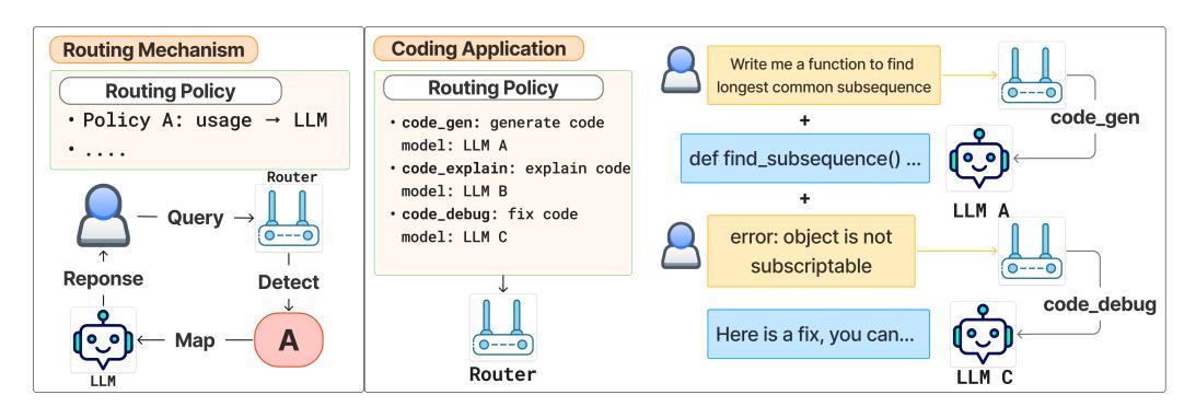Figure 2: Preference-aligned routing decouples policy selection $F$ from model assignment $T$. New models just edit $T$; new use cases are appended to $\mathcal{C}$. (source: Tran et al. 2025)

As a 1.5B model, Arch-Router runs in the tens of milliseconds on commodity GPUs and reports about 28× lower end-to-end latency than the closest commercial competitor under their setup, while matching or exceeding routing accuracy.

Two things matter most: routing fidelity is capped by policy quality (overlapping or ambiguous descriptions will confuse any router), and global outcomes still depend on the user’s $T$ mapping (accurate routing to a mismatched model is still suboptimal). This complements performance-based routers: when “quality” is subjective and organization-specific, encode it as policies and optimize $F$; when you trust a scalar quality predictor and care primarily about cost, optimize that score under a budget. A hybrid that uses preference-aligned $F$ with explicit cost/quality terms in $T$ or downstream escalation is natural.

Adaptive LLM Routing Under Budget Constraints treats routing as online learning with partial feedback (contextual bandits) plus explicit budget control. The idea is to learn a shared embedding space where query vectors and model vectors live, initialize it from human preference data, then adapt online from bandit feedback while enforcing a running cost budget. Let $L={l_1,\dots,l_k}$ be the model set. A query $q_t$ is embedded via $\phi$ and projected to $\psi(q_t)\in\mathbb{R}^{d_m}$. Each model $l$ has an embedding $\theta_l\in\mathbb{R}^{d_m}$. The expected reward under arm/model $a$ is a cosine similarity

\[\mathbb{E}[r_t\mid a,q_t]=\cos\!\big(\hat{\psi}(q_t),\hat{\theta}_a\big)=\hat{\psi}(q_t)^\top \hat{\theta}_a,\]

with unit-normalized $\hat{\cdot}$, which gives a linear bandit over $\psi(q_t)$

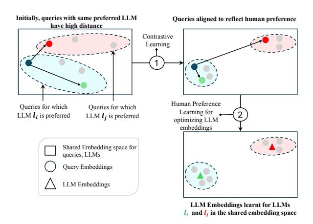Figure 3: 1) leverage human preference dataset to learn query embeddings which are aligned w.r.t. human preferences on query-LLM mapping. Then, in 2) learn LLM embeddings aligned with projected queries (source: Panda et al. 2025)

For Pretraining (preference prior), Using human preference tuples they first learn a query projection $\psi(q)=W\phi(q)+b$ via a triplet-style objective, then fix $W,b$ and learn model embeddings $\theta_l^{\text{pref}}$ by predicting the preferred model via a softmax over cosine scores. This stabilizes the shared space and provides a useful prior.

Online learning (PILOT). They instantiate a preference-prior informed LinUCB with

\[\tilde{\theta}_a^t=(A_a^t)^{-1} b_a^t,\quad A_a^0=\lambda_a I,\; b_a^0=\lambda_a \theta_a^{\text{pref}},\] \[A_a^t=A_a^{t-1}+\hat{\psi}(q_t)\hat{\psi}(q_t)^\top,\quad b_a^t=b_a^{t-1}+r_t\,\hat{\psi}(q_t).\]

At time $t$ they pick

\[a_t=\arg\max_a\;\Big(\cos\big(\hat{\psi}(q_t),\tilde{\theta}_a^t\big)+\alpha\sqrt{\hat{\psi}(q_t)^\top(A_a^t)^{-1}\hat{\psi}(q_t)}\Big).\]

The prior reduces regret when it is reasonably close to the true reward vector; the paper sketches an improvement over standard OFUL under a norm bound and gives the formal statement in the appendix.

Budget-aware routing. To enforce a total spend $B$ over $Q$ queries, they use an online cost policy modeled as an online multi-choice knapsack with thresholds. Let $z_t\in[0,1]$ denote current budget utilization. Eligible models satisfy

\[C_t^l \;\le\; \frac{\cos\!\big(\hat{\psi}(q_t),\hat{\theta}_l^t\big)} {\big(\tfrac{UB\cdot e}{LB}\big)^{z_t}\left(\tfrac{LB}{e}\right)},\]

using bounds $UB,LB$ on value-to-cost ratios. They also bin the $Q$ queries and allocate per-bin budgets with spillover to avoid under-spending in finite horizons. This puts cost under explicit online control without freezing the learning signal.

ROUTELLM studies the common binary case where we choose between a strong model (higher quality, higher cost) and a weak model (lower cost). The router is learned directly from human preference data with targeted augmentation for out-of-distribution evaluation. Let $\mathcal{M}\times{\text{strong}},\mathcal{M}\times{\text{weak}}$ be the classes. Given preference data

\[\mathcal{D}_{\text{pref}}=\{(q,l_{s,w})\},\quad l_{s,w}\in\{win_s,\ tie,\ win_w\},\]

they train a win prediction model $P_\theta(win_s\mid q)$ by maximizing

\[\max_{\theta}\ \sum_{(q,l_{s,w})\in \mathcal{D}_{\text{pref}}}\log P_\theta(l_{s,w}\mid q)\]

A threshold $\alpha\in[0,1]$ induces the routing rule

\[R^{\alpha}(q)= \begin{cases} \mathcal{M}_{\text{weak}}, & P_\theta(win_s\mid q)<\alpha,\\ \mathcal{M}_{\text{strong}}, & P_\theta(win_s\mid q)\ge \alpha, \end{cases}\]

and the router executes a single call

\[M_{R^{\alpha}}(q)= \begin{cases} M_s(q), & R^{\alpha}(q)=\mathcal{M}_{\text{strong}},\\ M_w(q), & R^{\alpha}(q)=\mathcal{M}_{\text{weak}}. \end{cases}\]

Here $\alpha$ trades cost for quality: larger $\alpha$ prefers the cheap model more often. Cost is the strong-call rate

\[c(M_{R^{\alpha}})=\frac{1}{|\mathcal{Q}|}\sum_{q}\mathbb{I}\{R^{\alpha}(q)=\mathcal{M}_{\text{strong}}\}\]

and performance is mean score

\[r(M_{R^{\alpha}})=\frac{1}{|\mathcal{Q}|}\sum_{q} s(M_{R^{\alpha}}(q))\]

They normalize performance via performance gap recovered (PGR)

\[\mathrm{PGR}(M_{R^{\alpha}})=\frac{r(M_{R^{\alpha}})-r(M_w)}{r(M_s)-r(M_w)}\]

and summarize the cost–quality curve by APGR (area under PGR vs. strong-call rate), approximated as

\[\mathrm{APGR}\approx \frac{1}{10}\sum_{i=1}^{10}\mathrm{PGR}(M_{R^{\alpha_i}})\]

Routers are instantiated in several ways but the idea stays simple. A similarity weighted Bradley Terry model reweights each preference pair by cosine similarity between query embeddings and solves a weighted BT objective, which is cheap and CPU-friendly. A matrix factorization model learns a bilinear score $\delta(M,q)$ and turns the difference into a win probability with a sigmoid. A BERT classifier fine-tunes a base encoder on win labels using the [CLS] representation. A causal LLM classifier fine-tunes an instruction-tuned Llama to emit label tokens and uses a softmax over win, tie, and weak. These transfer across unseen model pairs without retraining and remain well above random, which suggests the routers learn query features that predict relative wins in a stable way. They also quantify how similar the benchmark distribution is to the preference data using a max-similarity score

\[\mathcal{S}(B,\mathcal{D}_{\text{pref}})=\frac{1}{n}\sum_{i=1}^{n}\max_{1\le j\le m}\frac{b_i\cdot d_j}{\|b_i\|\,\|d_j\|}\]

which correlates with downstream performance and explains why the two targeted augmentations help. On cost and overhead they give a simple token-mix estimate: GPT-4 is about $24.7$/Mtok vs Mixtral about $0.24$/Mtok, routers reduce GPT-4 calls enough to realize around 2.5-3.7 times savings at high quality, with serving overhead small compared to generation and even the CPU-only method adding under about 0.4% of GPT-4 cost in their setup.